Expected Goals Prediction: How xG Improves Football Forecasts

What Expected Goals Prediction Means in Football Analytics

Expected goals prediction means using shot-quality probabilities to forecast future scoring, not just reviewing what the scoreboard said. Each shot receives a value from 0 to 1 based on historical conversion rates from similar chances.

A tap-in from six yards might be worth 0.45 xG. A weak shot from 30 yards might be 0.02. Team xG is the sum of those shot probabilities across the match, so five poor shots can still be less valuable than one clear chance.

That matters in forecasting because xG captures chance quality rather than possession, territory, or shot volume. Shot-based expected-goals models can outperform shot counts alone because quality carries more predictive information than volume, according to peer-reviewed sports analytics research.

On our 07:30 UTC model refresh, a 1-0 win with 0.55 xG is treated very differently from a 1-0 win with 2.10 xG.

Small number. Big signal.

How the Expected Goals Model Works Behind the Scenes

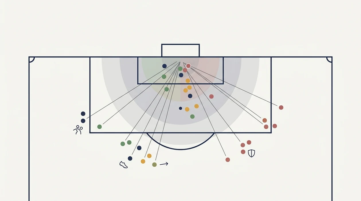
An expected goals model estimates shot probability by comparing a current shot with historical shots that had similar characteristics. The core inputs usually include shot location, angle to goal, body part, assist type, and defender pressure.

Modern xG models are often machine learning classifiers trained on hundreds of thousands of historical shots. The model learns which features raise or lower conversion probability. Academic football analytics research has shown that models using location, angle, body part, assist type, and defensive pressure estimate shot probability better than simpler shot-total approaches source.

Providers are not interchangeable. StatsBomb, Opta, and FBref can produce different xG numbers for the same match because their event definitions, tracking inputs, and model features differ. I’ve seen a comma-separated fixture file pass validation, then fail a calibration check because one provider coded a blocked shot differently.

Pre-Shot vs Post-Shot xG Models

Pre-shot xG measures chance quality before the shot is struck. Post-shot xG adds shot placement, so it is better for judging finishing and goalkeeping. For future forecasting, pre-shot xG usually carries the cleaner team-performance signal.

Five Facts Every Fan Needs About xG Prediction

Here are the five xG prediction facts worth keeping beside any match card or score forecast.

• xG assigns shot probability: Each shot gets a scoring probability, and a team’s match xG is the sum of those probabilities.
• xG is an input, not a crystal ball: It works best inside a broader model that also reads injuries, tactics, rest, and game state.
• xG differential points toward likely strength: Teams with stronger xG for minus xG against are often better future candidates, but variance still creates draws and upsets.
• xG supports multiple markets: It can improve match score prediction, BTTS predictions, and total-goals forecasts.
• Edges can close quickly: Once xG trends become visible in public numbers, market odds often adjust and reduce the forecasting advantage.

The practical takeaway is simple: xG helps explain process, not destiny. The model confidence badge can turn amber fast when a striker absence flashes in the lineup feed.

Before You Use xG Prediction

Before you use xG prediction, make sure the data is clean, comparable, and matched to the fixture context. A strong-looking trend can break quickly if the sample mixes providers, competitions, or team states.

1. Choose one xG source for the whole comparison window, because provider definitions and model features can move the same match total up or down.
2. Check team news before trusting the historical line. Suspensions, injuries, expected lineups, and late rotation can change the attacking baseline more than the last five-match average.
3. Separate competitions when the incentives differ. League xG, cup xG, and European xG should not always sit in one bucket if managers rotate heavily or protect a lead across two legs.
4. Confirm the xG type before feeding it into a forecast. Pre-shot xG is cleaner for team process, post-shot xG says more about finishing and goalkeeping, and mixed feeds can blur both signals.
5. Set a rolling minimum before reacting. Use a sample such as 6 to 10 matches so one wild red-card game or freak finishing night does not steer the whole prediction.

How to Use Expected Goals Prediction for Match Forecasts

Use xG prediction as a structured input, then test it against real outcomes and market prices. Single-match xG is noisy, so rolling samples matter more than one dramatic Saturday result.

1. Collect rolling xG for and xG against over at least 6 to 10 matches for each team.
2. Calculate xG differential by subtracting xG against from xG for over the same sample.
3. Compare xG-based expected scoreline to actual goals to flag possible finishing luck or goalkeeper overperformance.
4. Feed xG inputs into a broader AI prediction model alongside injuries, form, tactical setup, rest, and venue.
5. Validate xG-based forecasts against market odds or closing lines before treating any difference as useful.

For match result forecasts, xG differential should sit beside baseline rating and home advantage. For total-goals forecasts, combine both teams’ attacking xG and defensive xG allowed.

A useful football prediction report gives probabilities, not certainty. Good AI football prediction outputs deliver calibrated win, score, BTTS, and total-goals probabilities, not guaranteed winners.

Tools like AI Soccer Predictor can help structure those inputs, but the working still needs inspection.

Why xG Differential Predicts Future Results Better Than Goals

xG differential often predicts future results better than raw goals because it separates repeatable chance creation from finishing noise. In Premier League analysis, expected-goals differential showed strong predictive power for future match results source.

Raw goals can mislead over short windows. Penalties, deflections, goalkeeper errors, and one elite finish can inflate a scoreline without showing stable attacking quality. xG-based measures are better at separating team performance from finishing luck over small samples, according to the same research area.

Regression to the mean is the key mechanism. If a team scores 12 goals from 6.0 xG, the model does not assume that finishing rate will continue forever. It reruns the simulation closer to the underlying chance profile.

For win markets, xG differential is often more useful than recent goal difference because it measures the quality of the chances created and allowed.

Applying xG Prediction to BTTS and Over/Under Totals

xG translates into BTTS and over/under forecasts by estimating attacking output and defensive leakiness for both teams. Use xG-for to measure chance creation, and xG-against to measure the quality of chances a team allows.

BTTS likelihood rises when both teams consistently generate more than 1.0 xG and also concede usable chances. A 1.4 xG-for team facing a defence allowing 1.6 xG-against deserves a different BTTS probability than a side living on low-quality crosses.

For totals, sum both teams’ rolling xG averages and compare the number with the line. If the combined xG profile sits around 3.0, it supports over 2.5 predictions more than a combined profile near 2.1.

Many pages explain xG theory, then stop before the practical rule. The scoreline grid on a laptop only helps when it connects xG to thresholds, variance, and price.

Common Mistakes When Using Expected Goals Models for Prediction

The most common xG mistake is treating it as the score a team “deserved.” xG estimates chance quality; it does not rewrite the result or remove finishing skill, goalkeeping, or randomness.

Another error is confusing xG with possession or shots on target. A team can hold 62% possession and still create almost nothing. It can also land three shots on target from poor angles and produce a weak xG total.

Sample size causes plenty of bad forecasts. One match can swing because of a red card, a tactical mismatch, or a team protecting a lead from the 55th minute. Rolling averages are safer than one-match reactions.

Provider calibration also matters. A 1.75 xG number from one site may not equal 1.75 elsewhere. Before a model run, we flag provider changes the same way we flag stale kickoff times during international tournaments.

Context still counts. The captain missing from warm-up photos can matter more than last month’s xG trend.